pacman::p_load(lme4,haven,foreign, stargazer, texreg, lattice, sjPlot, dplyr, ggplot2, ggeffects) # paquetes a cargarPráctica 6: Interacción entre niveles
Correspondiente a la sesión del lunes, 26 de mayo de 2025
1 Cargar/instalar librerías
2 Ejemplo 1, datos HSB
2.1 Datos
mlm = read_dta("http://www.stata-press.com/data/mlmus3/hsb.dta")
dim(mlm)
names(mlm)
attach(mlm)
Tabla estadisticos descriptivos
stargazer(as.data.frame(mlm),title="Estadísticos descriptivos", type = "text")
Estadísticos descriptivos
===================================================
Statistic   N     Mean    St. Dev.    Min     Max
---------------------------------------------------
minority  7,185   0.275     0.446      0       1
female    7,185   0.528     0.499      0       1
ses       7,185  0.0001     0.779   -3.758   2.692
mathach   7,185  12.748     6.878   -2.832  24.993
size      7,185 1,056.862  604.172    100    2,713
sector    7,185   0.493     0.500      0       1
pracad    7,185   0.534     0.251    0.000   1.000
disclim   7,185  -0.132     0.944   -2.416   2.756
himinty   7,185   0.280     0.449      0       1
schoolid  7,185 5,277.898 2,499.578  1,224   9,586
mean      7,185  12.748     3.006    4.240  19.719
sd        7,185   6.198     0.864    3.541   8.481
sdalt     7,185   6.256     0.000    6.256   6.256
junk      7,185  47.316    48.898   0.00002 239.289
sdalt2    7,185  48.394     0.000   48.394  48.394
num       7,185  48.016    10.822     14      67
se        7,185   0.919     0.202    0.506   1.824
sealt     7,185   0.925     0.129    0.764   1.672
sealt2    7,185   1.028     0.144    0.850   1.859
t2        7,185  14.656    26.416    0.001  195.811
t2alt     7,185   8.538    11.063    0.001  52.825
pickone   7,185   0.022     0.148      0       1
mmses     7,185  0.0001     0.414   -1.194   0.825
mnses     7,185  0.0001     0.414   -1.194   0.825
xb        7,185  12.685     2.425    5.684  17.522
resid     7,185   0.062     6.459   -19.489 16.445
---------------------------------------------------
2.2 Modelos
- Revisar estructura variable para la interacción
str(mlm$sector)num [1:7185] 0 0 0 0 0 0 0 0 0 0 … - attr(*, “format.stata”)= chr “%8.0g”
table(mlm$sector)0 1 3642 3543
mlm$sector_f=as.factor(mlm$sector) # Cambiar a factor- Pendiente fija & aleatoria
reg_mlm3a = lmer(mathach ~ 1 + ses + sector_f +  mnses + (1 | schoolid),data=mlm)

# Con pendiente aleatoria
reg_mlm3b = lmer(mathach ~ 1 + ses + sector_f + mnses + (1 + ses | schoolid),data=mlm)- Devianza (ajuste comparativo pendiente fija vs aleatoria)
anova(reg_mlm3b,reg_mlm3a)Data: mlm
Models:
reg_mlm3a: mathach ~ 1 + ses + sector_f + mnses + (1 | schoolid)
reg_mlm3b: mathach ~ 1 + ses + sector_f + mnses + (1 + ses | schoolid)
npar AIC BIC logLik deviance Chisq Df Pr(>Chisq)
reg_mlm3a 6 46560 46602 -23274 46548
reg_mlm3b 8 46558 46613 -23271 46542 6.0463 2 0.04865 *
---
Signif. codes: 0 '***' 0.001 '**' 0.01 '*' 0.05 '.' 0.1 ' ' 1- Estimar modelo con interacción
reg_mlm3c = lmer(mathach ~ 1 + ses + sector_f + ses*sector_f + mnses +  (1 + ses | schoolid), data=mlm)
htmlreg(c(reg_mlm3a,reg_mlm3b, reg_mlm3c)) # screenreg() para visualización en R
<table class="texreg" style="margin: 10px auto;border-collapse: collapse;border-spacing: 0px;caption-side: bottom;color: #000000;border-top: 2px solid #000000;">
<caption>Statistical models</caption>
<thead>
<tr>
<th style="padding-left: 5px;padding-right: 5px;"> </th>
<th style="padding-left: 5px;padding-right: 5px;">Model 1</th>
<th style="padding-left: 5px;padding-right: 5px;">Model 2</th>
<th style="padding-left: 5px;padding-right: 5px;">Model 3</th>
</tr>
</thead>
<tbody>
<tr style="border-top: 1px solid #000000;">
<td style="padding-left: 5px;padding-right: 5px;">(Intercept)</td>
<td style="padding-left: 5px;padding-right: 5px;">12.13<sup>***</sup></td>
<td style="padding-left: 5px;padding-right: 5px;">12.04<sup>***</sup></td>
<td style="padding-left: 5px;padding-right: 5px;">12.20<sup>***</sup></td>
</tr>
<tr>
<td style="padding-left: 5px;padding-right: 5px;"> </td>
<td style="padding-left: 5px;padding-right: 5px;">(0.20)</td>
<td style="padding-left: 5px;padding-right: 5px;">(0.20)</td>
<td style="padding-left: 5px;padding-right: 5px;">(0.20)</td>
</tr>
<tr>
<td style="padding-left: 5px;padding-right: 5px;">ses</td>
<td style="padding-left: 5px;padding-right: 5px;">2.19<sup>***</sup></td>
<td style="padding-left: 5px;padding-right: 5px;">2.20<sup>***</sup></td>
<td style="padding-left: 5px;padding-right: 5px;">2.78<sup>***</sup></td>
</tr>
<tr>
<td style="padding-left: 5px;padding-right: 5px;"> </td>
<td style="padding-left: 5px;padding-right: 5px;">(0.11)</td>
<td style="padding-left: 5px;padding-right: 5px;">(0.12)</td>
<td style="padding-left: 5px;padding-right: 5px;">(0.14)</td>
</tr>
<tr>
<td style="padding-left: 5px;padding-right: 5px;">sector_f1</td>
<td style="padding-left: 5px;padding-right: 5px;">1.22<sup>***</sup></td>
<td style="padding-left: 5px;padding-right: 5px;">1.41<sup>***</sup></td>
<td style="padding-left: 5px;padding-right: 5px;">1.27<sup>***</sup></td>
</tr>
<tr>
<td style="padding-left: 5px;padding-right: 5px;"> </td>
<td style="padding-left: 5px;padding-right: 5px;">(0.31)</td>
<td style="padding-left: 5px;padding-right: 5px;">(0.31)</td>
<td style="padding-left: 5px;padding-right: 5px;">(0.30)</td>
</tr>
<tr>
<td style="padding-left: 5px;padding-right: 5px;">mnses</td>
<td style="padding-left: 5px;padding-right: 5px;">3.15<sup>***</sup></td>
<td style="padding-left: 5px;padding-right: 5px;">3.16<sup>***</sup></td>
<td style="padding-left: 5px;padding-right: 5px;">3.13<sup>***</sup></td>
</tr>
<tr>
<td style="padding-left: 5px;padding-right: 5px;"> </td>
<td style="padding-left: 5px;padding-right: 5px;">(0.38)</td>
<td style="padding-left: 5px;padding-right: 5px;">(0.39)</td>
<td style="padding-left: 5px;padding-right: 5px;">(0.38)</td>
</tr>
<tr>
<td style="padding-left: 5px;padding-right: 5px;">ses:sector_f1</td>
<td style="padding-left: 5px;padding-right: 5px;"> </td>
<td style="padding-left: 5px;padding-right: 5px;"> </td>
<td style="padding-left: 5px;padding-right: 5px;">-1.33<sup>***</sup></td>
</tr>
<tr>
<td style="padding-left: 5px;padding-right: 5px;"> </td>
<td style="padding-left: 5px;padding-right: 5px;"> </td>
<td style="padding-left: 5px;padding-right: 5px;"> </td>
<td style="padding-left: 5px;padding-right: 5px;">(0.21)</td>
</tr>
<tr style="border-top: 1px solid #000000;">
<td style="padding-left: 5px;padding-right: 5px;">AIC</td>
<td style="padding-left: 5px;padding-right: 5px;">46565.83</td>
<td style="padding-left: 5px;padding-right: 5px;">46563.47</td>
<td style="padding-left: 5px;padding-right: 5px;">46532.06</td>
</tr>
<tr>
<td style="padding-left: 5px;padding-right: 5px;">BIC</td>
<td style="padding-left: 5px;padding-right: 5px;">46607.11</td>
<td style="padding-left: 5px;padding-right: 5px;">46618.51</td>
<td style="padding-left: 5px;padding-right: 5px;">46593.98</td>
</tr>
<tr>
<td style="padding-left: 5px;padding-right: 5px;">Log Likelihood</td>
<td style="padding-left: 5px;padding-right: 5px;">-23276.92</td>
<td style="padding-left: 5px;padding-right: 5px;">-23273.74</td>
<td style="padding-left: 5px;padding-right: 5px;">-23257.03</td>
</tr>
<tr>
<td style="padding-left: 5px;padding-right: 5px;">Num. obs.</td>
<td style="padding-left: 5px;padding-right: 5px;">7185</td>
<td style="padding-left: 5px;padding-right: 5px;">7185</td>
<td style="padding-left: 5px;padding-right: 5px;">7185</td>
</tr>
<tr>
<td style="padding-left: 5px;padding-right: 5px;">Num. groups: schoolid</td>
<td style="padding-left: 5px;padding-right: 5px;">160</td>
<td style="padding-left: 5px;padding-right: 5px;">160</td>
<td style="padding-left: 5px;padding-right: 5px;">160</td>
</tr>
<tr>
<td style="padding-left: 5px;padding-right: 5px;">Var: schoolid (Intercept)</td>
<td style="padding-left: 5px;padding-right: 5px;">2.37</td>
<td style="padding-left: 5px;padding-right: 5px;">2.43</td>
<td style="padding-left: 5px;padding-right: 5px;">2.34</td>
</tr>
<tr>
<td style="padding-left: 5px;padding-right: 5px;">Var: Residual</td>
<td style="padding-left: 5px;padding-right: 5px;">37.02</td>
<td style="padding-left: 5px;padding-right: 5px;">36.78</td>
<td style="padding-left: 5px;padding-right: 5px;">36.79</td>
</tr>
<tr>
<td style="padding-left: 5px;padding-right: 5px;">Var: schoolid ses</td>
<td style="padding-left: 5px;padding-right: 5px;"> </td>
<td style="padding-left: 5px;padding-right: 5px;">0.47</td>
<td style="padding-left: 5px;padding-right: 5px;">0.07</td>
</tr>
<tr style="border-bottom: 2px solid #000000;">
<td style="padding-left: 5px;padding-right: 5px;">Cov: schoolid (Intercept) ses</td>
<td style="padding-left: 5px;padding-right: 5px;"> </td>
<td style="padding-left: 5px;padding-right: 5px;">0.29</td>
<td style="padding-left: 5px;padding-right: 5px;">0.18</td>
</tr>
</tbody>
<tfoot>
<tr>
<td style="font-size: 0.8em;" colspan="4"><sup>***</sup>p < 0.001; <sup>**</sup>p < 0.01; <sup>*</sup>p < 0.05</td>
</tr>
</tfoot>
</table>2.3 Plot
plot_model(reg_mlm3c, type = "int")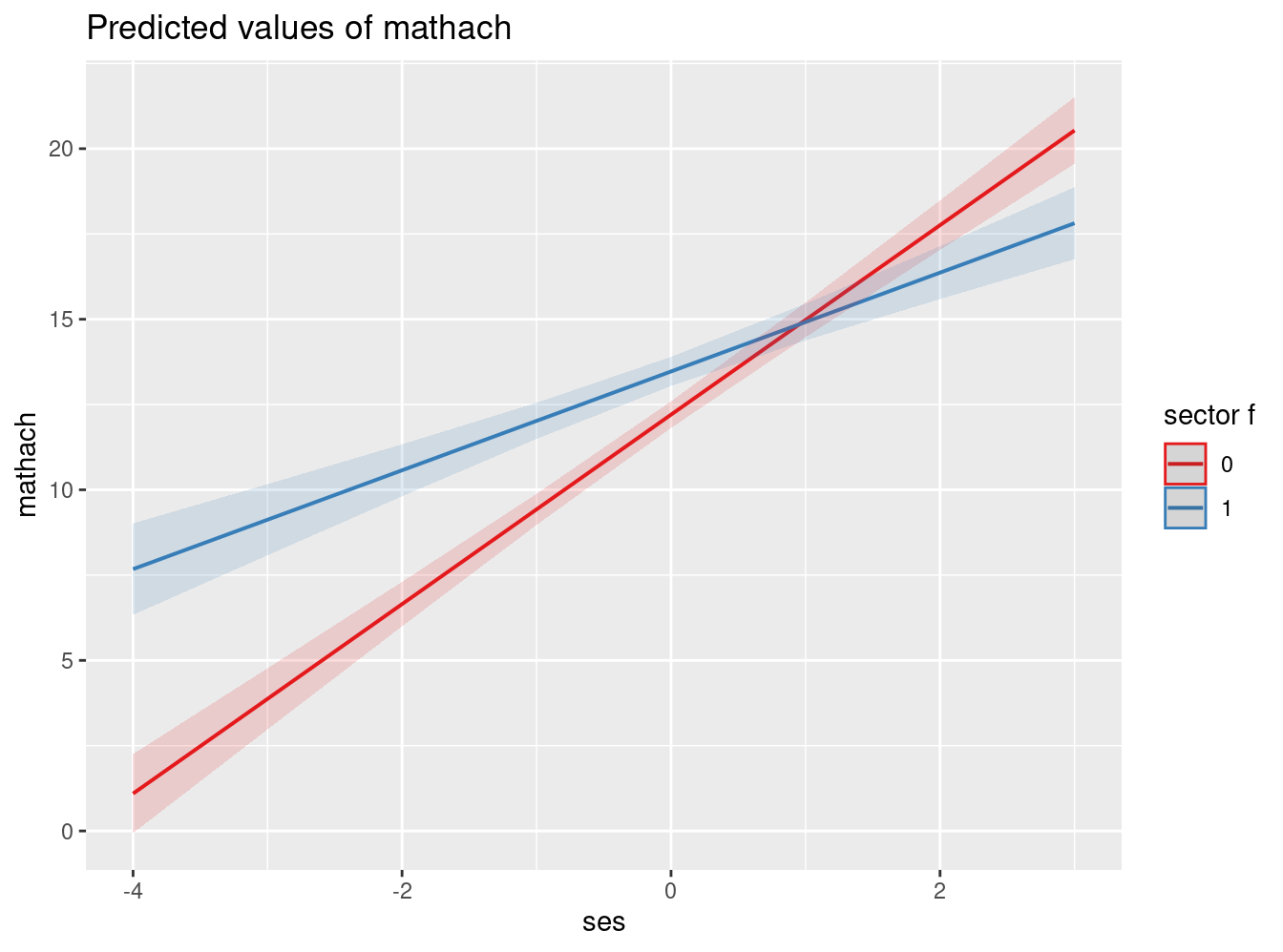
3 Ejemplo Aguinis
Link a paper aquí
Planteamiento general:
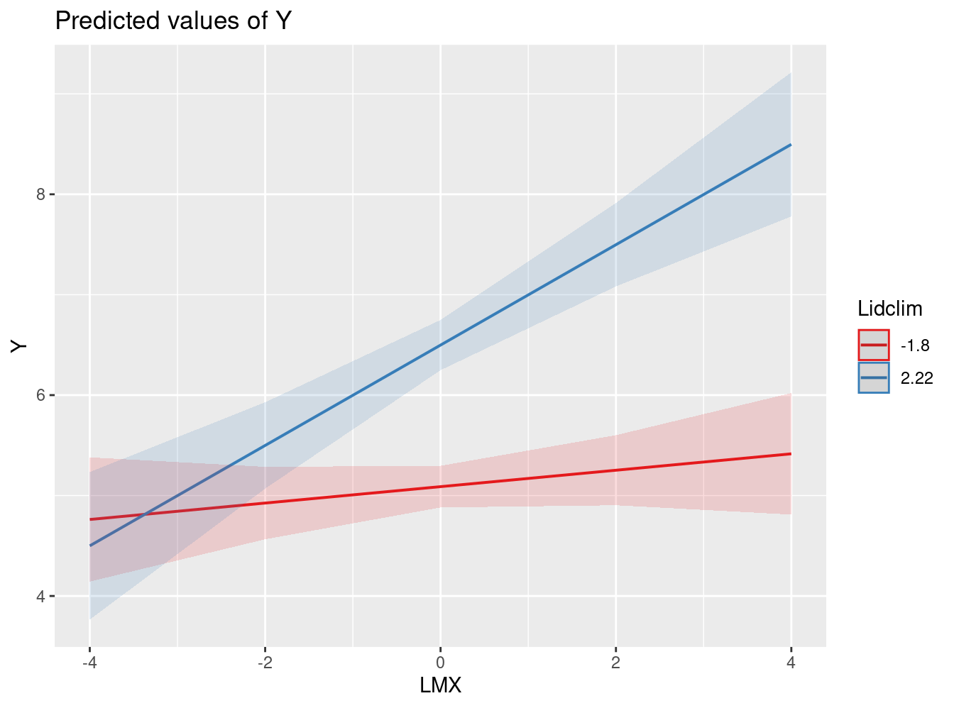
” Overall, Chen et al.’s theoretical model predicted that employees who report higher LMX (i.e., a better relationship with their leader) will feel more empowered (i.e., they have the autonomy and capability to perform meaning- ful work that can affect their organization). In addition, Chen et al.’s model included the hypothesis that the team-level variable leadership climate (i.e., ambient leadership behaviors directed at the team as a whole) would also affect individual-level empowerment positively. Moreover, Chen et al. hypothesized that the relationship between LMX and empowerment would be moderated by leadership climate such that the relationship would be stronger for teams with a better leadership climate.” (p.1492)
- Preguntas e hipótesis:
Lower-level direct effects. Does a lower-level predictor X (i.e., Level 1 or L1 predictor) have an effect on a lower-level outcome variable Y (i.e., L1 outcome)? Specifically regarding our illus- tration, there is an interest in testing whether LMX, as perceived by subordinates, predicts individual empowerment. Note that LMX scores are collected for each individual worker (i.e., there is no aggregation of such scores for the purpose of testing the presence of a lower-level direct effect).
Cross-level direct effects. Does a higher-level predictor W (i.e., Level 2 or L2 predictor) have an effect on an L1 outcome variable Y? Specifically, we would like to assess whether L2 variable leadership climate predicts L1 outcome individual empowerment.
Cross-level interaction effects. Does the nature or strength of the relationship between two lower-level variables (e.g., L1 predictor X and L1 outcome Y) change as a function of a higher- level variable W? Referring back to our substantive illustration, we are interested in testing the hypothesis that the relationship between LMX and individual empowerment may vary as a function of (i.e., is moderated by) the degree of leadership climate such that the relationship will be stronger for teams with more positive leadership climate and weaker for teams with less positive leadership climate.
3.1 Datos
exdata=read.csv("https://multinivel.netlify.app/practicas/data/aguinis_JOM.csv", header = TRUE, sep = ",")
stargazer(exdata, type = "text")
============================================
Statistic  N   Mean  St. Dev.   Min    Max
--------------------------------------------
l1id      630 3.500   1.709      1      6
l2id      630 53.000  30.334     1     105
X         630 4.800   1.500    0.221  8.731
Xbarj     630 4.800   0.793    3.319  6.907
Wj        630 4.770   0.700    2.966  6.987
cat       630 0.505   0.500      0      1
Y         630 5.720   0.900    2.739  8.381
Xc        630 0.000   1.273   -3.904  3.865
XcWj      630 -0.000  6.196   -22.683 18.487
Wjc       630 -0.000  0.700   -1.804  2.217
--------------------------------------------- Rename variables para que sean más coherentes con el ejemplo
exdata <- exdata %>% rename(LMX=Xc,Lidclim=Wjc)Variables relevantes
- l2id: id de nivel 2, equipos de trabajo
- LMX: quality of leader–member exchange
- Lidclim: clima de liderazgo en el equipo
- Y: variable dependiente, empoderamiento individual
3.2 Modelos
- Modelo Nulo e ICC
lmm.fit1=lmer(Y ~ 1 + (1|l2id), data=exdata,REML=F)
summary(lmm.fit1)
Linear mixed model fit by maximum likelihood ['lmerMod']
Formula: Y ~ 1 + (1 | l2id)
Data: exdata
AIC BIC logLik deviance df.resid
1643.0 1656.4 -818.5 1637.0 627
Scaled residuals:
Min 1Q Median 3Q Max
-2.96708 -0.61992 -0.00518 0.60150 2.88977
Random effects:
Groups Name Variance Std.Dev.
l2id (Intercept) 0.09494 0.3081
Residual 0.71378 0.8449
Number of obs: 630, groups: l2id, 105
Fixed effects:
Estimate Std. Error t value
(Intercept) 5.72000 0.04513 126.7reghelper::ICC(lmm.fit1)[1] 0.1173919- Modelo con predictores fijos
lmm.fit2=lmer(Y ~1 + LMX + Lidclim +(1|l2id),data=exdata,REML=F)
screenreg(lmm.fit2)
==================================
                       Model 1
----------------------------------
(Intercept)               5.72 ***
                         (0.04)
LMX                       0.28 ***
                         (0.02)
Lidclim                   0.35 ***
                         (0.05)
----------------------------------
AIC                    1487.64
BIC                    1509.87
Log Likelihood         -738.82
Num. obs.               630
Num. groups: l2id       105
Var: l2id (Intercept)     0.06
Var: Residual             0.56
==================================
*** p < 0.001; ** p < 0.01; * p < 0.05- Pendiente aleatoria
lmm.fit3=lmer(Y ~1 + LMX + Lidclim +(1 + LMX|l2id), data=exdata,REML=F)
summary(lmm.fit3)
Linear mixed model fit by maximum likelihood ['lmerMod']
Formula: Y ~ 1 + LMX + Lidclim + (1 + LMX | l2id)
Data: exdata
AIC BIC logLik deviance df.resid
1483.5 1514.6 -734.7 1469.5 623
Scaled residuals:
Min 1Q Median 3Q Max
-3.0693 -0.5814 -0.0309 0.5965 3.5938
Random effects:
Groups Name Variance Std.Dev. Corr
l2id (Intercept) 0.06802 0.2608
LMX 0.02529 0.1590 -0.09
Residual 0.51438 0.7172
Number of obs: 630, groups: l2id, 105
Fixed effects:
Estimate Std. Error t value
(Intercept) 5.72000 0.03827 149.478
LMX 0.26958 0.02829 9.530
Lidclim 0.35570 0.05468 6.505
Correlation of Fixed Effects:
(Intr) LMX
LMX -0.034
Lidclim 0.000 -0.001Deviance
anova(lmm.fit2,lmm.fit3)Data: exdata
Models:
lmm.fit2: Y ~ 1 + LMX + Lidclim + (1 | l2id)
lmm.fit3: Y ~ 1 + LMX + Lidclim + (1 + LMX | l2id)
npar AIC BIC logLik deviance Chisq Df Pr(>Chisq)
lmm.fit2 5 1487.6 1509.9 -738.82 1477.6
lmm.fit3 7 1483.5 1514.6 -734.75 1469.5 8.1422 2 0.01706 *
---
Signif. codes: 0 '***' 0.001 '**' 0.01 '*' 0.05 '.' 0.1 ' ' 1- Modelo con interacción entre niveles
lmm.fit4=lmer(Y ~1 + LMX*Lidclim + (1 + LMX|l2id), data=exdata, REML=F)
screenreg(lmm.fit4)
======================================
                           Model 1
--------------------------------------
(Intercept)                   5.72 ***
                             (0.04)
LMX                           0.27 ***
                             (0.03)
Lidclim                       0.35 ***
                             (0.05)
LMX:Lidclim                   0.10 **
                             (0.04)
--------------------------------------
AIC                        1478.19
BIC                        1513.76
Log Likelihood             -731.10
Num. obs.                   630
Num. groups: l2id           105
Var: l2id (Intercept)         0.07
Var: l2id LMX                 0.02
Cov: l2id (Intercept) LMX    -0.00
Var: Residual                 0.52
======================================
*** p < 0.001; ** p < 0.01; * p < 0.05
3.3 Reporte final
- Tabla
screenreg(list(lmm.fit1, lmm.fit2, lmm.fit3, lmm.fit4))
=============================================================================
                           Model 1      Model 2      Model 3      Model 4
-----------------------------------------------------------------------------
(Intercept)                   5.72 ***     5.72 ***     5.72 ***     5.72 ***
                             (0.05)       (0.04)       (0.04)       (0.04)
LMX                                        0.28 ***     0.27 ***     0.27 ***
                                          (0.02)       (0.03)       (0.03)
Lidclim                                    0.35 ***     0.36 ***     0.35 ***
                                          (0.05)       (0.05)       (0.05)
LMX:Lidclim                                                          0.10 **
                                                                    (0.04)
-----------------------------------------------------------------------------
AIC                        1643.04      1487.64      1483.50      1478.19
BIC                        1656.38      1509.87      1514.62      1513.76
Log Likelihood             -818.52      -738.82      -734.75      -731.10
Num. obs.                   630          630          630          630
Num. groups: l2id           105          105          105          105
Var: l2id (Intercept)         0.09         0.06         0.07         0.07
Var: Residual                 0.71         0.56         0.51         0.52
Var: l2id LMX                                           0.03         0.02
Cov: l2id (Intercept) LMX                              -0.00        -0.00
=============================================================================
*** p < 0.001; ** p < 0.01; * p < 0.05
En html
htmlreg(list(lmm.fit1, lmm.fit2, lmm.fit3, lmm.fit4),
    custom.model.names = c("Nulo","Pendiente <br> fija","Pendiente <br> Aleatoria", "Interacción"),
    custom.coef.names = c("Intercepto", "LMX $(\\gamma_{10})$" ,"Clima liderazgo $(\\gamma_{01})$", "LMX*Clima $(\\gamma_{11})$"),
    custom.gof.names=c(NA,NA,NA,NA,NA,
                   "Var: l2id ($\\tau_{00}$)",
                   "Var: Residual ($\\sigma^2$)",
                   "Var: l2id LMX ($\\tau_{11}$)",
                   "Cov: l2id (Intercept) LMX ($\\tau_{01}$)"),
    custom.note = "%stars. Errores estándar en paréntesis",
    caption="Replicacion Tabla Aguinis",
    caption.above=TRUE,
    digits=3,
doctype = FALSE)| Nulo |
Pendiente fija |
Pendiente Aleatoria |
Interacción | |
|---|---|---|---|---|
| Intercepto | 5.720*** | 5.720*** | 5.720*** | 5.720*** |
| (0.045) | (0.038) | (0.038) | (0.038) | |
| LMX \((\gamma_{10})\) | 0.279*** | 0.270*** | 0.269*** | |
| (0.023) | (0.028) | (0.027) | ||
| Clima liderazgo \((\gamma_{01})\) | 0.351*** | 0.356*** | 0.351*** | |
| (0.055) | (0.055) | (0.055) | ||
| LMX*Clima \((\gamma_{11})\) | 0.104** | |||
| (0.037) | ||||
| AIC | 1643.040 | 1487.641 | 1483.499 | 1478.192 |
| BIC | 1656.377 | 1509.870 | 1514.619 | 1513.758 |
| Log Likelihood | -818.520 | -738.821 | -734.749 | -731.096 |
| Num. obs. | 630 | 630 | 630 | 630 |
| Num. groups: l2id | 105 | 105 | 105 | 105 |
| Var: l2id (\(\tau_{00}\)) | 0.095 | 0.060 | 0.068 | 0.068 |
| Var: Residual (\(\sigma^2\)) | 0.714 | 0.563 | 0.514 | 0.516 |
| Var: l2id LMX (\(\tau_{11}\)) | 0.025 | 0.019 | ||
| Cov: l2id (Intercept) LMX (\(\tau_{01}\)) | -0.004 | -0.004 | ||
| ***p < 0.001; **p < 0.01; *p < 0.05. Errores estándar en paréntesis | ||||
- Interaction Plot
plot_model(lmm.fit4, type = "int")